Linear Regression

Chapter 1: Linear Regression

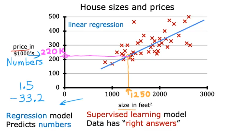
Linear Regression is a fundamental algorithm used to predict a continuous numerical value. We start by building a model that can predict housing prices based on the size of the house.

Notation

To understand the model, let's first define our notation:

• Training Set: The data used to train the model.
• $x$: The input variable or feature. (e.g., size of a house).
• $y$: The output variable or target. This is the true value we want to predict (e.g., price of the house).
• $m$: The total number of training examples in the dataset.
• $(x, y)$: A single training example.
• $(x^{(i)}, y^{(i)})$: The i-th training example in the dataset (e.g., $(x^{(1)}, y^{(1)})$ is the first example).

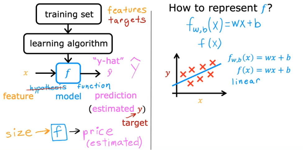
The Model (Hypothesis)

The model is a function, which we'll call $f$, that takes an input $x$ and produces a prediction $\hat{y}$ (pronounced "y-hat").

• $f$: The model or hypothesis function.
• $\hat{y}$: The predicted output from the model.

For Univariate Linear Regression (linear regression with one variable), the model $f$ is a linear function:

Here:

• $w$ is the weight of the model (determines the slope of the line).
• $b$ is the bias of the model (determines the y-intercept).
• $w$ and $b$ are also called the parameters of the model.

Lab: Model Representation in Python

Here is a simple implementation of the linear regression model using Python, NumPy, and Matplotlib.

import numpy as np
import matplotlib.pyplot as plt
plt.style.use('./deeplearning.mplstyle')

# x_train is the input variable (size in 1000 square feet)
# y_train is the target (price in 1000s of dollars)
x_train = np.array([1.0, 2.0])
y_train = np.array([300.0, 500.0])
print(f"x_train = {x_train}")
print(f"y_train = {y_train}")

# m is the number of training examples
# We can get m from the shape of the array or using len()
m = x_train.shape[0]
print(f"Number of training examples is: {m}")

# Let's look at a single training example
i = 0 # Change this to 1 to see the second example
x_i = x_train[i]
y_i = y_train[i]
print(f"(x^({i}), y^({i})) = ({x_i}, {y_i})")

# Plot the data points to visualize them
plt.scatter(x_train, y_train, marker='x', c='r')
plt.title("Housing Prices")
plt.ylabel('Price (in 1000s of dollars)')
plt.xlabel('Size (1000 sqft)')
plt.show()

# Let's define our model parameters w and b
w = 200
b = 100
print(f"w: {w}")
print(f"b: {b}")

def compute_model_output(x, w, b):
    """
    Computes the prediction of a linear model.
    Args:
      x (ndarray (m,)): Data, m examples 
      w,b (scalar)    : model parameters  
    Returns
      f_wb (ndarray (m,)): model prediction
    """
    m = x.shape[0]
    f_wb = np.zeros(m)
    for i in range(m):
        f_wb[i] = w * x[i] + b
    return f_wb

# Let's compute the predictions for our training data
tmp_f_wb = compute_model_output(x_train, w, b,)

# Plot our model's prediction against the actual values
plt.plot(x_train, tmp_f_wb, c='b', label='Our Prediction')
plt.scatter(x_train, y_train, marker='x', c='r', label='Actual Values')
plt.title("Housing Prices")
plt.ylabel('Price (in 1000s of dollars)')
plt.xlabel('Size (1000 sqft)')
plt.legend()
plt.show()

# Predict the price of a 1200 sqft house
x_i = 1.2
cost_1200sqft = w * x_i + b 
print(f"Predicted price for a 1200 sqft house: ${cost_1200sqft:.0f} thousand dollars")

The Cost Function

To find the best possible line to fit our data, we need a way to measure how well our model is performing. This is where the Cost Function, denoted as $J(w, b)$, comes in.

The cost function measures the difference (or error) between the model's predictions ($\hat{y}$) and the actual target values ($y$). For linear regression, the most common cost function is the Squared Error Cost Function.

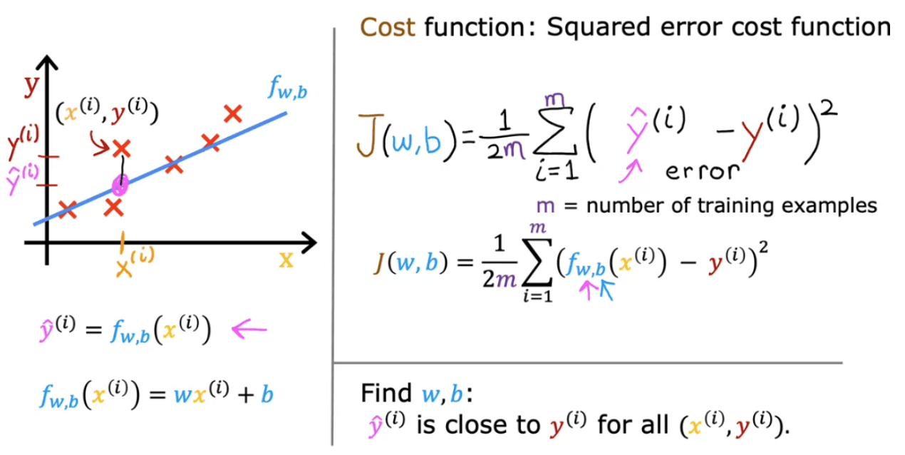
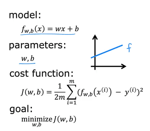
Goal: Find the values of $w$ and $b$ that minimize the cost function $J(w, b)$.

Cost Function Intuition

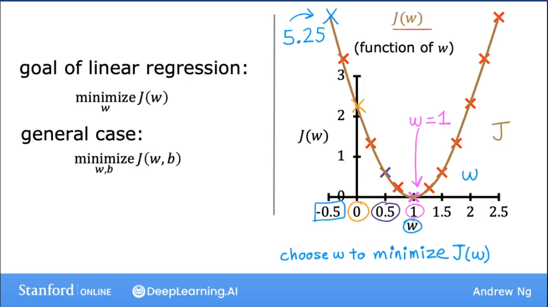
Let's simplify our model to build intuition. Assume $b = 0$, so our model is just $f_w(x) = w*x$. The line must pass through the origin.

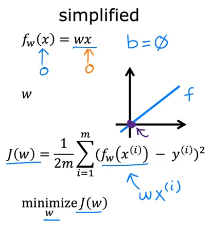
Now, our cost function $J$ only depends on $w$: $J(w)$. We can plot $J(w)$ versus $w$.

• $f_w(x)$ is a function of $x$ (the input).
• $J(w)$ is a function of $w$ (the parameter).

The plots below show how changing $w$ affects both the model's prediction line and the value of the cost function $J(w)$.

Model $f_w(x)$ (Prediction Line)	Cost Function $J(w)$
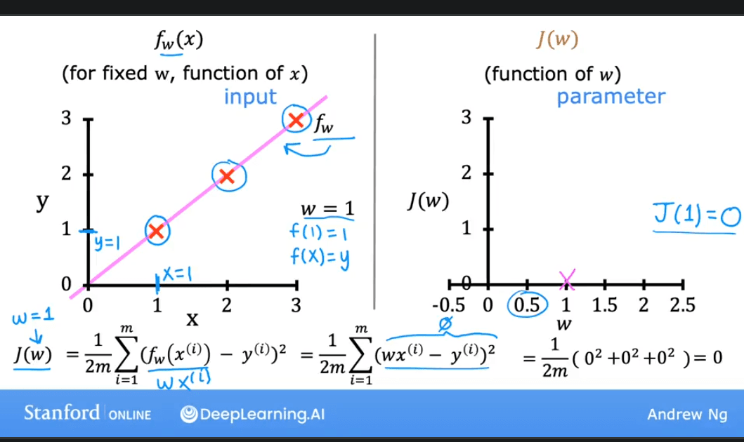	The cost $J(w)$ is 0 when $w=1$, which is the optimal value.
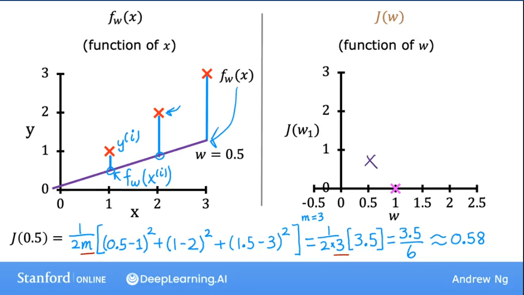	The cost $J(w)$ is higher when $w=0.5$.
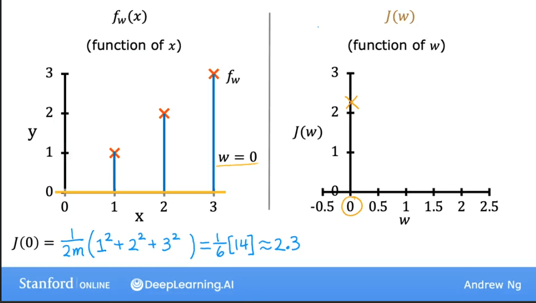	The cost $J(w)$ is also higher when $w=1.5$.

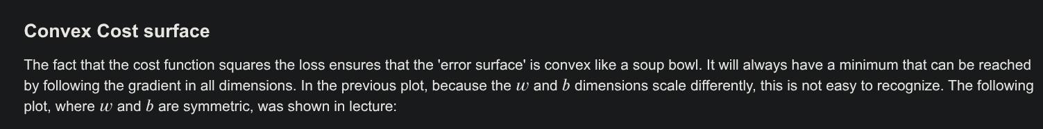
Plotting $J(w)$ for a range of $w$ values gives us a parabola (a bowl shape). Our goal is to find the value of $w$ at the bottom of the bowl, where the cost is at its minimum.

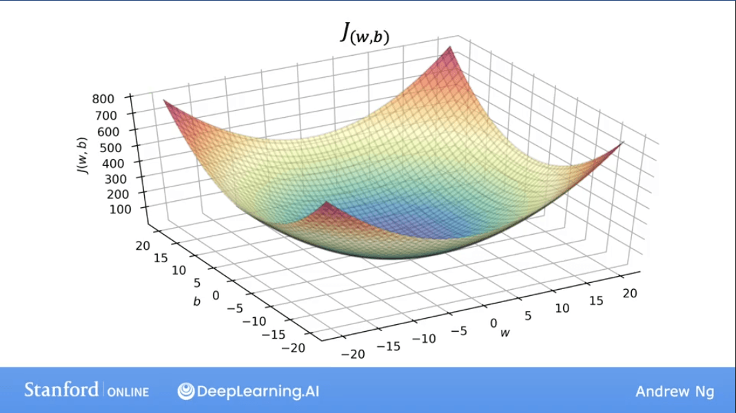
Visualizing the Full Cost Function $J(w, b)$

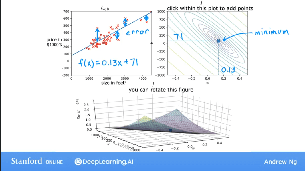
When we re-introduce the bias term $b$, our cost function $J(w, b)$ depends on two parameters. Visualizing this requires a 3D plot.

The 3D surface plot of $J(w, b)$ forms a "bowl" shape. The lowest point of the bowl represents the minimum cost, and the $w$ and $b$ values at that point are our optimal parameters.

A more convenient way to visualize this in 2D is using a Contour Plot. Imagine slicing the 3D bowl horizontally at different heights. The outlines of these slices, when viewed from above, form the contour plot.

Each ellipse on the contour plot represents a set of $(w, b)$ pairs that result in the same cost $J(w, b)$. The center of the innermost ellipse is the point of minimum cost.

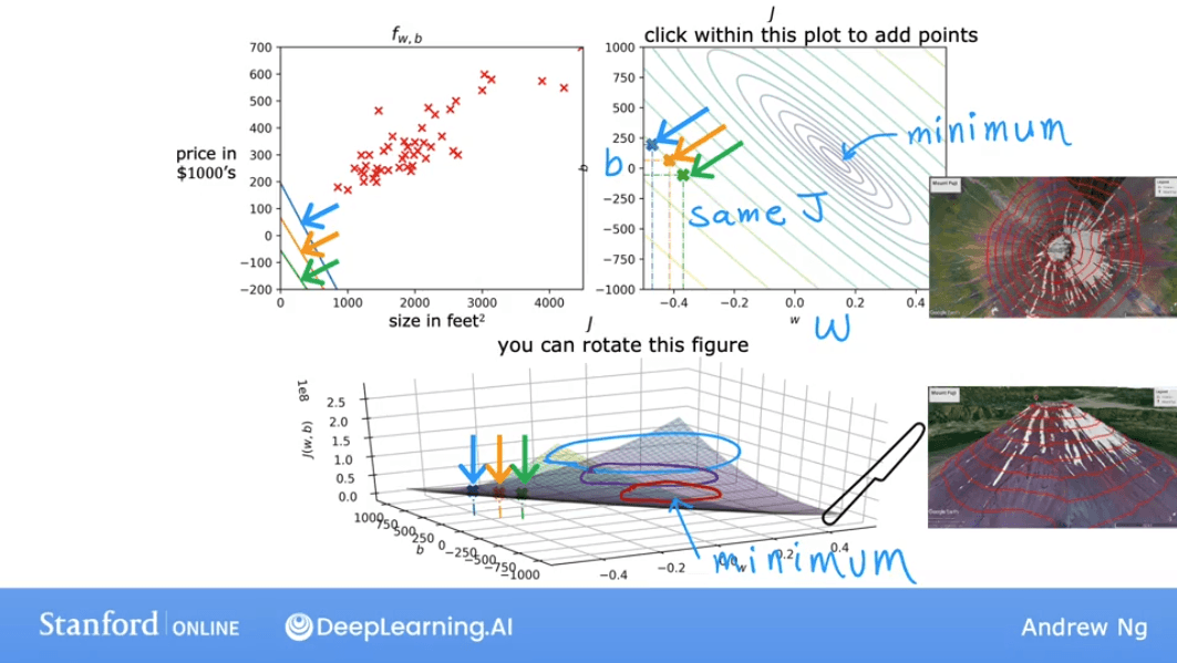
As we move the point $(w, b)$ on the contour plot, the prediction line $f(x)$ on the data plot changes. The goal is to find the center of the ellipses, which corresponds to the best-fit line.

Lab: Visualizing the Cost Function

This lab provides interactive plots to explore how $w$ and $b$ affect the cost $J(w, b)$.

import numpy as np
%matplotlib widget
import matplotlib.pyplot as plt
from lab_utils_uni import plt_intuition, plt_stationary, plt_update_onclick, soup_bowl
plt.style.use('./deeplearning.mplstyle')

# Training data
x_train = np.array([1.0, 2.0])           # (size in 1000 square feet)
y_train = np.array([300.0, 500.0])       # (price in 1000s of dollars)

def compute_cost(x, y, w, b): 
    """
    Computes the cost function for linear regression.    
    Args:
      x (ndarray (m,)): Data, m examples 
      y (ndarray (m,)): target values
      w,b (scalar)    : model parameters  
    
    Returns
        total_cost (float): The cost of using w,b as the parameters for linear regression
                            to fit the data points in x and y.
    """
    # number of training examples
    m = x.shape[0] 
    
    cost_sum = 0 
    for i in range(m): 
        f_wb = w * x[i] + b   
        cost = (f_wb - y[i]) ** 2  
        cost_sum = cost_sum + cost  
    total_cost = (1 / (2 * m)) * cost_sum  

    return total_cost

# Interactive plot to build intuition on cost function with respect to w (b is fixed)
plt_intuition(x_train, y_train)

# More complex dataset
x_train = np.array([1.0, 1.7, 2.0, 2.5, 3.0, 3.2])
y_train = np.array([250, 300, 480, 430, 630, 730])

# Interactive plot showing cost contour and 3D surface
plt.close('all') 
fig, ax, dyn_items = plt_stationary(x_train, y_train)
updater = plt_update_onclick(fig, ax, x_train, y_train, dyn_items)

# Plot of a generic bowl-shaped cost function
soup_bowl()

Summary from Notes

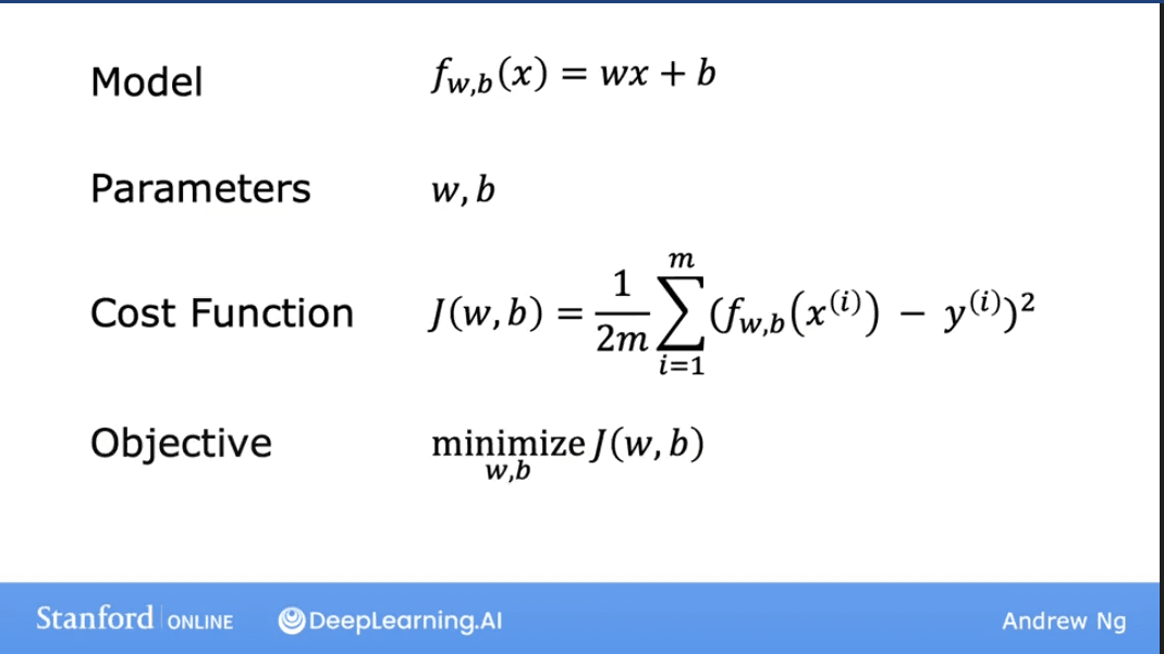
The core formulas for the Linear Regression model and its cost function are:

1. Model (Hypothesis): The prediction $f(x)$ for a single input $x$.

   $$f_{w,b}(x^{(i)}) = w * x^{(i)} + b$$

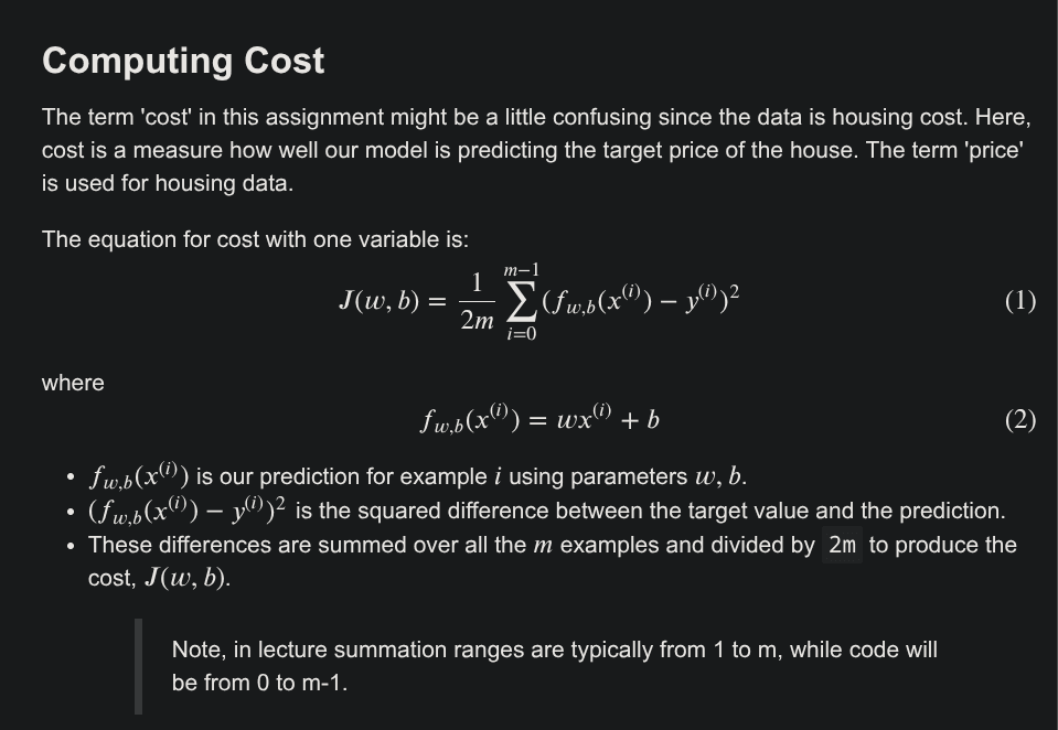
2. Cost Function: $J(w, b)$ measures the average squared error over all $m$ training examples.

   $$J(w, b) = \frac{1}{2m} \sum_{i=1}^{m} \left( f_{w,b}(x^{(i)}) - y^{(i)} \right)^2$$

   Where:

   • $Σ$ is the summation symbol, summing from $i=1$ to $m$.
   • $(f_w,b(x^{(i)}) - y^{(i)})$ is the error for the i-th example.
   • The error is squared to penalize larger errors more and to ensure the cost is always positive.
   • $\frac{1}{2m}$ is a scaling factor. The $\frac{1}{m}$ gives the average error, and the $\frac{1}{2}$ simplifies the math for the derivative later on.