Classification with Logistic Regression
Classification is a type of supervised learning where the the model's goal is to predict which category a new observation belongs to.
Classification
Classification problems are everywhere. The goal is to assign an input to one of a discrete number of categories or classes.
Examples: History
- Is this email spam?
(Yes/No) - Is the transaction fraudulent?
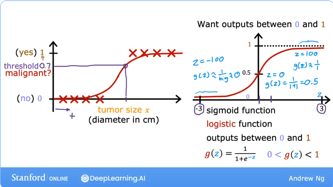
(Yes/No) - Is this tumor malignant?
(Yes/No)
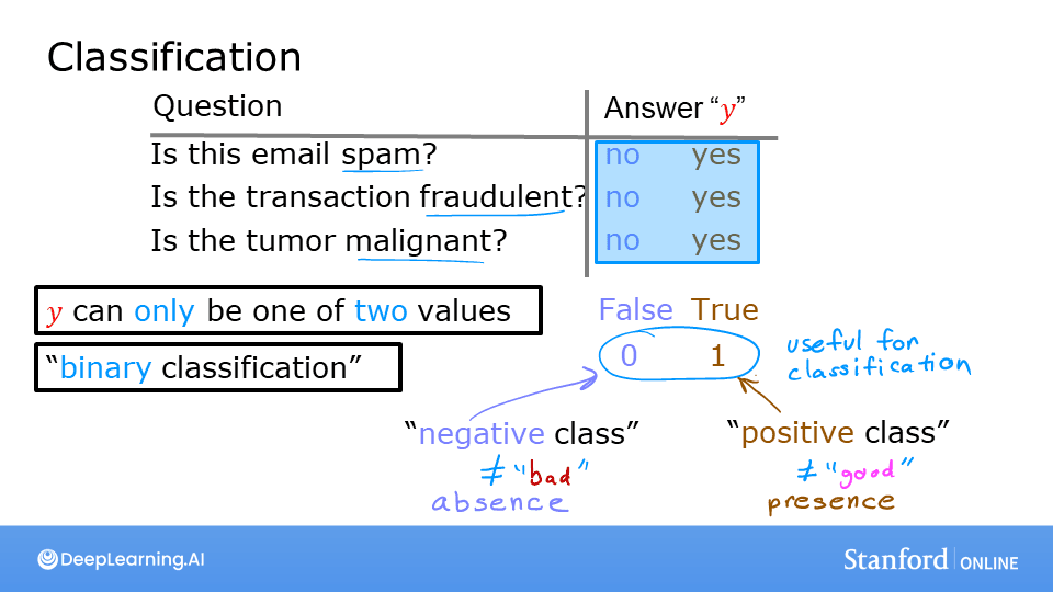
Binary Classification
This is the simplest form of classification, where the output variable can only take on one of two possible values or classes.
Notation: We often use specific terms and numerical representations for these two classes:
- Negative Class (0): Represents the absence of something (e.g.,
no,false,not spam,benign tumor). - Positive Class (1): Represents the presence of something (e.g.,
yes,true,spam,malignant tumor).
Why Not Use Linear Regression?
At first glance, one might think of using linear regression for classification problems. After all, if the output is just 0 or 1, why not fit a line and see if the output is closer to 0 or 1? However, this approach has significant flaws.
When we use linear regression, the model fits a straight line to the data. If we set a classification threshold (e.g., at 0.5), it might seem to work for a simple dataset. But, this approach is very sensitive to outliers.
If we add an outlier to the training data, the best-fit line of the linear regression model will shift significantly. This shift also moves the decision threshold, leading to misclassification of existing data points. Additionally, linear regression can output values much greater than 1 or less than 0, which doesn't make sense for a probability estimate.
 As seen above, adding a single outlier point on the right causes the linear model's decision boundary to shift, resulting in an incorrect prediction for the point that was previously classified correctly.
Lab: Demonstrating the Problem with Linear Regression
Goal
In this lab, you will contrast regression and classification and see why linear regression is not ideal for classification tasks.
Code
import numpy as np
%matplotlib widget
import matplotlib.pyplot as plt
from lab_utils_common import dlc, plot_data
from plt_one_addpt_onclick import plt_one_addpt_onclick
plt.style.use('./deeplearning.mplstyle')
# Example Data
x_train = np.array([0., 1, 2, 3, 4, 5])
y_train = np.array([0, 0, 0, 1, 1, 1])
X_train2 = np.array([[0.5, 1.5], [1,1], [1.5, 0.5], [3, 0.5], [2, 2], [1, 2.5]])
y_train2 = np.array([0, 0, 0, 1, 1, 1])
# Plotting the data
pos = y_train == 1
neg = y_train == 0
fig,ax = plt.subplots(1,2,figsize=(8,3))
#plot 1, single variable
ax[0].scatter(x_train[pos], y_train[pos], marker='x', s=80, c = 'red', label="y=1")
ax[0].scatter(x_train[neg], y_train[neg], marker='o', s=100, label="y=0", facecolors='none',
edgecolors=dlc["dlblue"],lw=3)
ax[0].set_ylim(-0.08,1.1)
ax[0].set_ylabel('y', fontsize=12)
ax[0].set_xlabel('x', fontsize=12)
ax[0].set_title('one variable plot')
ax[0].legend()
#plot 2, two variables
plot_data(X_train2, y_train2, ax[1])
ax[1].axis([0, 4, 0, 4])
ax[1].set_ylabel('$x_1$', fontsize=12)
ax[1].set_xlabel('$x_0$', fontsize=12)
ax[1].set_title('two variable plot')
ax[1].legend()
plt.tight_layout()
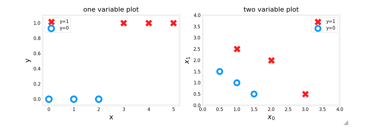
plt.show()Observations
Plots of classification data often use symbols to indicate the outcome. Here, 'X' represents the positive class (1) and 'O' represents the negative class (0).
Linear Regression Approach
Running linear regression on this data initially seems to work if we apply a 0.5 threshold. Predictions match the data.
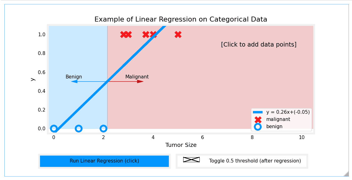
However, adding more 'malignant' data points on the far right and re-running the regression causes the model to shift. This leads to incorrect predictions for points that were previously classified correctly.
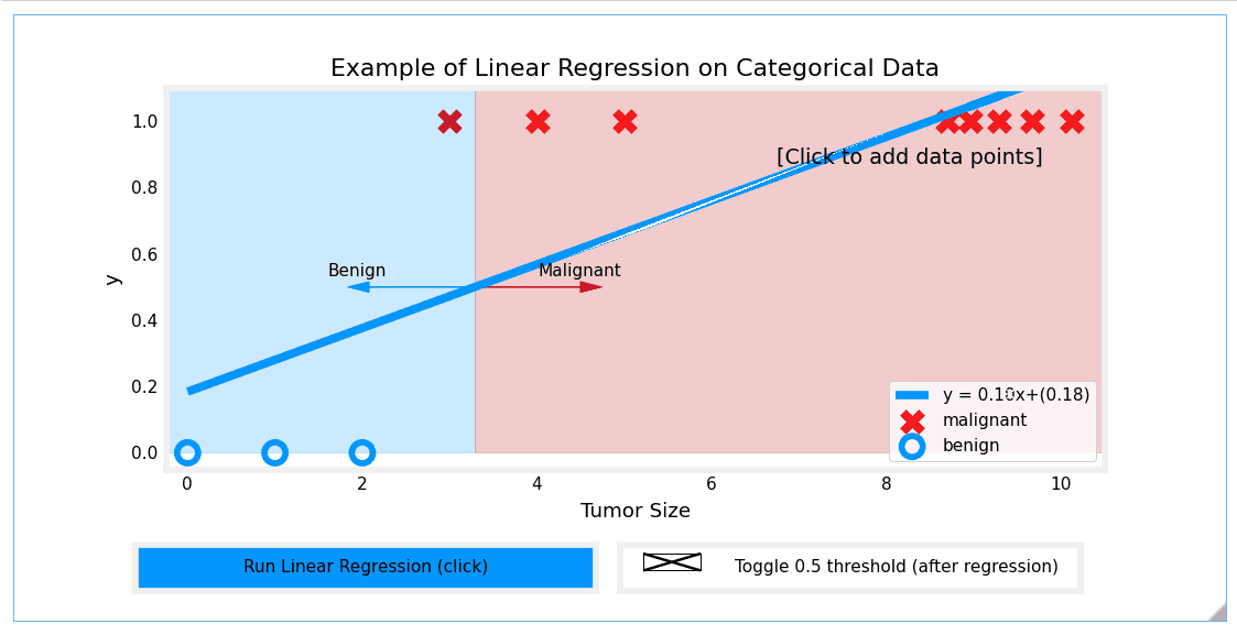
Conclusion
This lab demonstrates that a linear model is insufficient for categorical data. We need a model whose output is always between 0 and 1 and which is less sensitive to outliers. This brings us to Logistic Regression.
Logistic Regression
Logistic Regression is one of the most popular and widely used classification algorithms. It is a go-to method for binary classification problems, despite its name suggesting it's a regression technique.
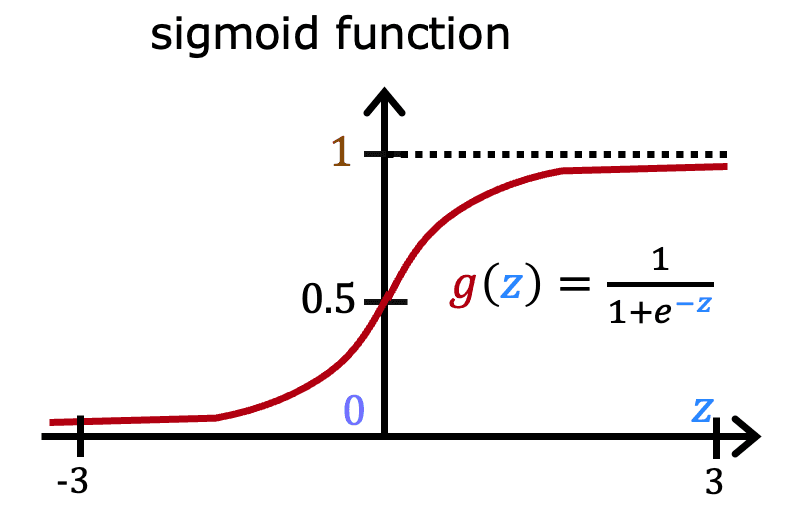
The Sigmoid Function (or Logistic Function)
The core of logistic regression is the Sigmoid Function, denoted as . This function takes any real-valued number and "squashes" it into a value between 0 and 1.
The formula is:
Where is Euler's number (approximately 2.718).
- When is a large positive number, is close to 0, so is close to 1.
- When is a large negative number, is a very large number, so is close to 0.
- When , , so is exactly 0.5.
The Logistic Regression Model
The model itself combines the linear regression formula with the sigmoid function. The linear part calculates a value , which is then passed to the sigmoid function to produce a probability.
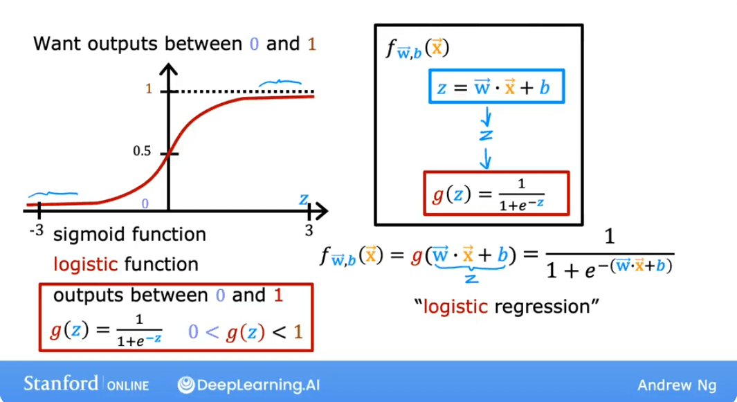
The output of this model, , is interpreted as the probability that the output is 1, given the input and parameters and .
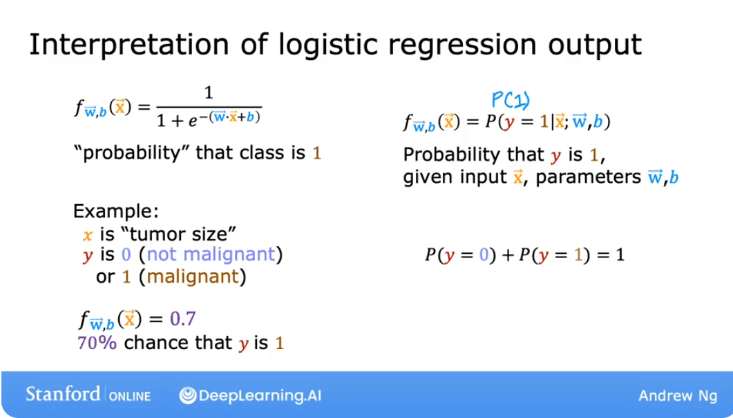
This can be written formally as:
Real-World Application: A variation of logistic regression was a key driver behind early online advertising systems, deciding which ads to show to which users to maximize the probability of a click.
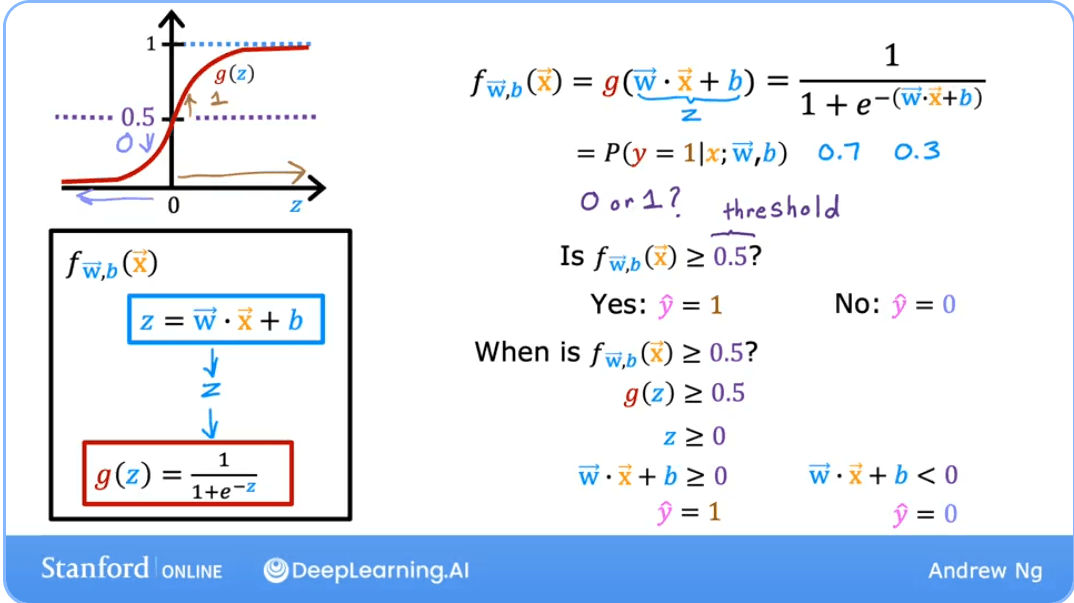
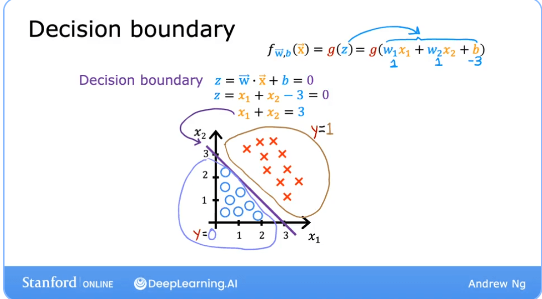
The Decision Boundary
The decision boundary is the line or surface that separates the different classes predicted by the model. It's the threshold where the model switches from predicting one class to another.
For logistic regression, we typically make a prediction as follows: Predict if:
Predict if:
Since the sigmoid function only when its input , the decision boundary corresponds to the line where:
This expands to:
This equation defines the decision boundary. Any point that makes this expression positive will be classified as 1, and any point that makes it negative will be classified as 0.
For a model with two features (, ), the decision boundary is a line given by:
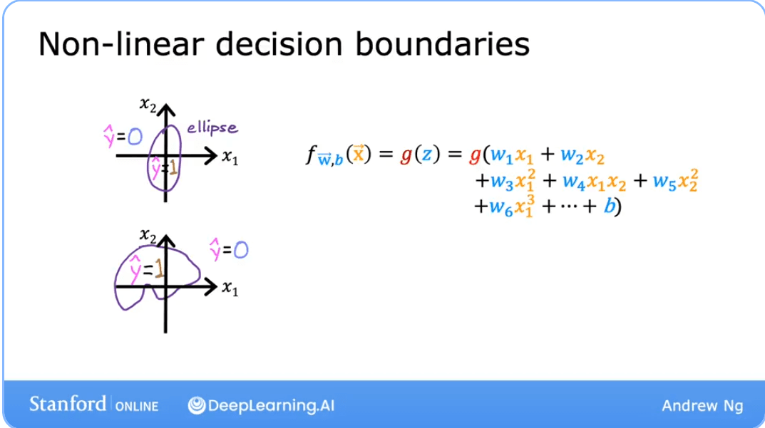
Complex (Non-Linear) Decision Boundaries
Logistic regression can also model complex, non-linear relationships by using polynomial features. Instead of just using and , we can create new features from the original ones, like , , , etc.
The model's internal calculation then becomes:
By setting this more complex argument to zero, we can create more complex decision boundaries, such as circles or other curved shapes. The decision boundary is still linear in the parameter space but is non-linear in the feature space.

Food for thought: Let's say you are creating a tumor detection algorithm. The model outputs a probability that a tumor is malignant. A specialist will later inspect any tumors flagged by your algorithm. What value should you use for a threshold?
- A. High, say a threshold of 0.9?
- B. Low, say a threshold of 0.2?
Answer: B. You would not want to miss a potential tumor (a false negative), so it's safer to use a low threshold. A specialist will review the output, which helps mitigate the impact of any false positives (cases where the model flags a benign tumor). This highlights that the classification threshold does not always have to be 0.5 and should be chosen based on the problem's context.
Lab: Logistic Regression and Decision Boundaries
Goals
- Explore the sigmoid function.
- Understand how a trained logistic regression model makes predictions.
- Plot the decision boundary for a logistic regression model.
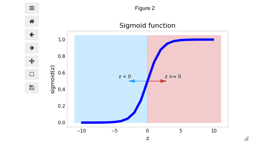
Part 1: The Sigmoid Function
The numpy.exp() function is used to compute . Let's implement the sigmoid function and visualize it.
import numpy as np
%matplotlib widget
import matplotlib.pyplot as plt
from lab_utils_common import plot_data, sigmoid, draw_vthresh
plt.style.use('./deeplearning.mplstyle')

# Sigmoid function implementation
# Note: The 'sigmoid' function is often imported from a utility file in labs.
def sigmoid(z):
    """
    Compute the sigmoid of z
    Args:
        z (ndarray): A scalar, numpy array of any size.
    Returns:
        g (ndarray): sigmoid(z), with the same shape as z
    """
    g = 1/(1+np.exp(-z))
    return g

# Plot sigmoid(z) over a range of values from -10 to 10
z = np.arange(-10,11)

fig,ax = plt.subplots(1,1,figsize=(5,3))
# Plot z vs sigmoid(z)
ax.plot(z, sigmoid(z), c="b")

ax.set_title("Sigmoid function")
ax.set_ylabel('sigmoid(z)')
ax.set_xlabel('z')
draw_vthresh(ax,0)
As you can see from the plot, when:
This is the key to our decision rule.
Part 2: Plotting a Decision Boundary
Let's use a sample training dataset with two features.
# Dataset
X = np.array([[0.5, 1.5], [1,1], [1.5, 0.5], [3, 0.5], [2, 2], [1, 2.5]])
y = np.array([0, 0, 0, 1, 1, 1]).reshape(-1,1)

# Plot data
fig,ax = plt.subplots(1,1,figsize=(4,4))
plot_data(X, y, ax)

ax.axis([0, 4, 0, 3.5])
ax.set_ylabel('$x_1$')
ax.set_xlabel('$x_0$')
plt.show()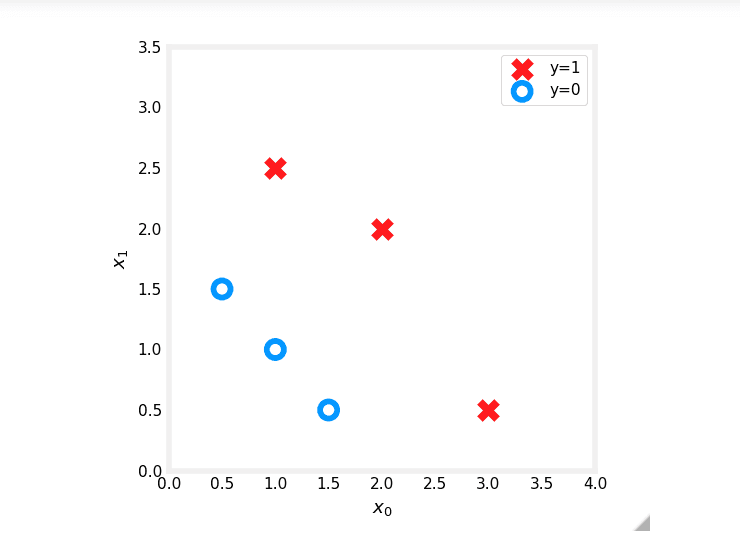
Now, suppose you've already trained a logistic regression model and found the optimal parameters to be , , . The model is:
The model predicts if:
The decision boundary is the line where this expression is exactly zero:
which we can rewrite as:
Let's plot this line on our data.
# Choose values for x0 between 0 and 6
x0 = np.arange(0,6)

# Calculate the corresponding x1 for the decision boundary
x1 = 3 - x0

fig,ax = plt.subplots(1,1,figsize=(5,4))
# Plot the decision boundary
ax.plot(x0, x1, c="b")
ax.axis([0, 4, 0, 3.5])

# Fill the region below the line, where the prediction is y=0
ax.fill_between(x0, x1, alpha=0.2)

# Plot the original data
plot_data(X,y,ax)
ax.set_ylabel(r'$x_1$')
ax.set_xlabel(r'$x_0$')
plt.show()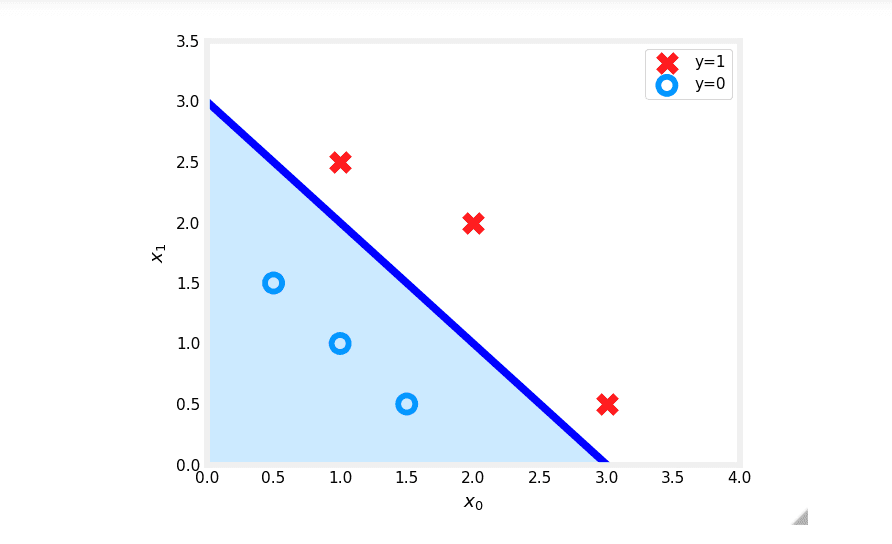
In the plot above:
- The blue line represents the decision boundary .
- The shaded region represents where . Any point in this region is classified as .
- The region above the line is where . Any point on or above the line is classified as .
This visualization clearly shows how the logistic regression model separates the two classes in the feature space.
Practice Quiz
Question 1: Which is an example of a classification task?
- A. Based on a patient's age and blood pressure, determine how much blood pressure medication (measured in milligrams) the patient should be prescribed.
- B. Based on a patient's blood pressure, determine how much blood pressure medication (a dosage measured in milligrams) the patient should be prescribed.
- C. Based on the size of each tumor, determine if each tumor is malignant (cancerous) or not.
Answer: C. This task predicts one of two classes, malignant or not malignant. The other options are regression tasks as they predict a continuous value (milligrams).
Question 2: Recall the sigmoid function is:
If is a large positive number, what is ?
- A. will be near 0.5
- B. will be near zero (0)
- C. is near one (1)
- D. is near negative one (-1)
Answer: C. If is a large positive number (e.g., 100), becomes a very small positive number (close to 0). So, becomes approximately:
Question 3: A cat photo classification model predicts 1 if it's a cat, and 0 if it's not. For a particular photo, the logistic regression model outputs . Which of these would be a reasonable criterion to predict if it's a cat?
- A. Predict it is a cat if
- B. Predict it is a cat if
- C. Predict it is a cat if
- D. Predict it is a cat if
Answer: C. We interpret as the probability that the photo is of a cat. A standard approach is to predict "cat" when this probability is greater than or equal to a 0.5 threshold.
Question 4: True/False: No matter what features you use (including if you use polynomial features), the decision boundary learned by logistic regression will be a linear decision boundary.
- A. True
- B. False
Answer: B. False. As explained in the "Non-Linear Decision Boundaries" section, using polynomial features (e.g., ) allows logistic regression to learn complex, non-linear decision boundaries in the original feature space.